Greener Journal of Economics and Accountancy Vol. 9(1), pp. 1-9, 2021 ISSN: 2354-2357 Copyright ©2021, the copyright of this article is retained by the author(s) https://gjournals.org/GJEA

Modeling and Forecasting Botswana’s Growth Domestic Product (GDP) per Capita

Nyoni, Thabani¹; Muchingami, Lovemore²; Olebogeng Mokgware³; Joe Jazi⁴; Georgina Mwantembe⁵

¹Department of Economics, University of Zimbabwe. Email: nyonithabani35@ gmail. com

²Snr Lecturer Department of Banking & Finance, BA ISAGO University, lavmuch@ gmail. com

³Department of Risk Management, Insurance and Actuarial Science, BA ISAGO University. Email. Olebogang.mkgware@ baisago.ac. bw

⁴Department of Entrepreneurship, BA ISAGO University. Email.Joe.jazi@ baisago.ac. bw

⁵Business Management, BA ISAGO University. Email: georgina.mwantembe@ baisago. ac.bw

ARTICLE INFO	ABSTRACT
Article No.: 041819073 Type: Research	Gross Domestic Product (GDP) per capita is regarded as one of the key signals of economic performance which may also be a benchmark for comparing living standards for different citizens across borders. There may be growth in real GDP without any improvement in real GDP per capita. Having this and other exogenous factors in concern, this research paper employed the Box-Jenkins ARIMA Methodology to analyse GDP per capita in Botswana from 1960 to 2017. The ADF tests show that Botswana GDP per capita data is I (1). Based on the AIC, the study presents the ARIMA (3, 2, 3) model. The diagnostic tests further show that the presented model is not only stable but also suitable. Ceteris paribus, the results of the study indicate that living standards in Botswana may absolutely continue to improve over the next decade. Four (4) policy recommendations were deduced from this research which the Botswana economic policy makers may consider in an effort to promote and maintain the much needed better living standards for all Batswana.
Accepted: 26/04/2017 Published: 31/05/2021
*Corresponding Author Muchingami, Lovemore E-mail: lavmuch@ gmail.com
Keywords: Botswana; Forecasting; GDP per capita

1.0 INTRODUCTION

The issue of gross domestic product (GDP) has become topical as it forms the prime worry in the macroeconomics fraternity. Policy makers and analysts are continually assessing the state of the economy since it is perceived to be one of the primary aggregate indicators used to measure the healthiness of any economy. Economic growth can be referred to as a sustained increase in per capita national output or net national product over a comprehensive period of time. A sustainable economic growth mainly rest on a country’s ability to invest and make a well-organized and productive resource endowment (Nyoni & Bonga, 2017f).

GDP per see does not reflect the overall state of the standard of living or well-being of a country, however, GDP per capita is often considered to reveal the condition of the average citizen in any country. To this end, GDP per capita in Botswana recorded at 7523.22 US dollars in 2017 which is equivalent to 60 percent of the world's average.  GDP per capita averaged 3427.73 USD from 1960 - 2017, recording the highest rate of 7574.30 USD in 2014 and lowest of 390.80 USD in 1960 (tradingeconomics.com). During the same period, Botswana gained a high middle income status as rated by the World Bank and UNDP Human Resource Development Index (Maipose & Matsheka, 2009). In Africa, the country was ranked top in terms of governance and transparency indices as reflected by political stability and constitutional democracy (Honde & Abraha, 2015).

This remarkable growth was attributed to prudent economic policies and mining sector contributions, which proved to be an important variable of growth in Botswana (IMF,2017). The sector contributed 24.5% to the country’s GDP in 2013. This makes Botswana a success story of Africa, with a strong government commitment to policies and a regulatory environment that foster private sector development (Todaro, 2012). Just like any other economy, the country requires a reliable, consistent and accurate GDP forecasts to conduct a progressive monetary and fiscal policies. Hence, this research attempts to model and forecast GDP per capita for the period 1960-2017.

2.0 LITERATURE REVIEW

In comparing the power of forecasting between ARIMA models and Artificial Neural Networks (ANN), Okasha and Yaseen (2013) agreed that the Box-Jenkins, ARIMA models proved to be more accurate than the Artificial Neural Network (ANN) making it an alternative to the Box-Jenkins approach. Using an econometric ANN model, Junoh (2004) modeled and forecasted GDP growth in Malaysia (1995-2000), found out that the ANN has an increased potential to predict GDP growth based on knowledge-based economy indicators compared to the Box-Jenkins approach. Lu (2009), in China; forecasted GDP using ARIMA models with annual data from 1962 to 2008 and noted that the ARIMA (4, 1, 0) model was the optimal model. In India, Bipasha & Bani (2012) forecasted GDP growth rates based on ARIMA models using annual data from 1959 to 2011 and established that the ARIMA (1, 2, 2) model was the optimal model to forecast GDP growth in India. In Greece, Dritsaki (2015) looked at real GDP basing on the Box-Jenkins ARIMA approach during the period 1980 – 2013 and noted that the ARIMA (1, 1, 1) model was the optimal model. In the case of Kenya, Wabomba et al (2016); modeled and forecasted GDP basing on ARIMA models with an annual data set ranging from 1960 to 2012 and concluded that the ARIMA (2, 2, 2) model was the optimal model for modeling GDP in Kenya.

3.0 MATERIALS & METHODS

3.1 ARIMA Models

ARIMA models are often considered as delivering more accurate forecasts than econometric techniques (Song et al, 2003b). ARIMA models outperform multivariate models in forecasting performance (du Preez & Witt, 2003). Overall performance of ARIMA models is superior to that of the naïve models and smoothing techniques (Goh & Law, 2002). ARIMA models were developed by Box and Jenkins in the 1970s and their approach of identification, estimation and diagnostics is based on the principle of parsimony (Asteriou & Hall, 2007). The mathematical formulation of the ARIMA (p, d, q) model using lag polynomials can be simply written as:

Where p and q are orders of the autoregressive (AR) and moving average (MA) components respectively and d is the number of times the series is differenced.

3.2 The Box – Jenkins Methodology

The first step towards model selection is to difference the series in order to achieve stationarity. Once this process is over, the researcher will then examine the correlogram in order to decide on the appropriate orders of the AR and MA components. It is important to highlight the fact that this procedure (of choosing the AR and MA components) is biased towards the use of personal judgement because there are no clear – cut rules on how to decide on the appropriate AR and MA components. Therefore, experience plays a pivotal role in this regard. The next step is the estimation of the tentative model, after which diagnostic testing shall follow. Diagnostic checking is usually done by generating the set of residuals and testing whether they satisfy the characteristics of a white noise process. If not, there would be need for model re – specification and repetition of the same process; this time from the second stage. The process may go on and on until an appropriate model is identified (Nyoni, 2018i).

4.0 Data Collection

This research work is hinged on 58 observations of annual GDP per capita in Botswana, from 1960 to 2017. Data was collected from the World Bank online database.

4.1 Diagnostic Tests & Model Evaluation

4.1.1Stationarity Tests: Graphical Analysis

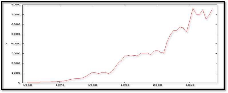
Figure 1

The Botswana GDP per capita variable, as shown above is not stationary because it is trending upwards and this implies that its mean is changing over time and thus its varience is not constant over time.

4.1.2 The Correlogram in Levels

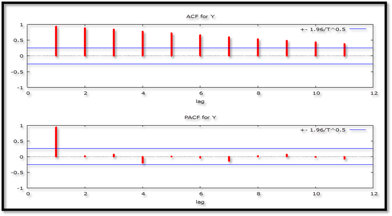
Figure 2

4.1.3 The ADF Test

Table 1: Levels-intercept

Variable	ADF Statistic	Probability	Critical Values		Conclusion
Y	1.295578	0.9983	-3.560019	@1%	Not stationary
			-2.917650	@5%	Not stationary
			-2.596689	@10%	Not stationary

Table 2: Levels-trend & intercept

Variable	ADF Statistic	Probability	Critical Values		Conclusion
Y	-2.022603	0.5766	-4.127338	@1%	Not stationary
			-3.490662	@5%	Not stationary
			-3.173943	@10%	Not stationary

Table 3: without intercept and trend & intercept

Variable	ADF Statistic	Probability	Critical Values		Conclusion
Y	2.541447	0.9970	-2.606163	@1%	Not stationary
			-1.946654	@5%	Not stationary
			-1.613122	@10%	Not stationary

Figures 2 and tables 1 – 3, all indicate the non-stationarity of GDP per capita in levels. Thus Y is not I (0).

4.1.4 The Correlogram (at 1^st Differences)

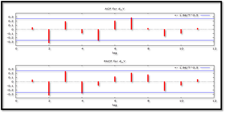
Figure 3

Table 4: 1^st Difference-intercept

Variable	ADF Statistic	Probability	Critical Values		Conclusion
Y	-4.503592	0.0006	-3.560019	@1%	Stationary
			-2.917650	@5%	Stationary
			-2.596689	@10%	Stationary

Table 5: 1^st Difference-trend & intercept

Variable	ADF Statistic	Probability	Critical Values		Conclusion
Y	-5.021871	0.0008	-4.140858	@1%	Stationary
			-3.496960	@5%	Stationary
			-3.177579	@10%	Stationary

Table 6: 1^st Difference-without intercept and trend & intercept

Variable	ADF Statistic	Probability	Critical Values		Conclusion
Y	-2.882143	0.0047	-2.608490	@1%	Stationary
			-1.946996	@5%	Stationary
			-1.612924	@10%	Stationary

Figure 3 as well as tables 4 – 6, all show that the Botswana GDP per capita series became stationary after taking first differences; therefore, it’s I (1).

4.2 Evaluation of ARIMA models (without a constant)

Table 7

Model	AIC	U	ME	MAE	RMSE	MAPE
ARIMA (1, 1, 1)	839.9019	0.89648	107.56	227.93	362.18	9.6045
ARIMA (2, 1, 1)	839.8412	0.94968	125.54	222.42	355.6	7.3849
ARIMA (3, 1, 1)	836.7766	0.87654	86.698	214.22	338.87	9.3593
ARIMA (4, 1, 1)	838.1568	0.88295	95.013	213.4	336.71	9.4365
ARIMA (4, 1, 0)	836.3743	0.88418	97.428	212.98	337.47	9.4365
ARIMA (3, 1, 0)	836.9577	0.87648	83.069	215.25	346.11	9.32248
ARIMA (0, 1, 1)	842.8361	0.85898	95.404	230.55	379.05	9.2927
ARIMA (0, 1, 2)	839.7101	0.91968	119.14	226.61	361.8	9.7583
ARIMA (2, 1, 2)	830.9423	0.88362	104.73	205.8	316.24	9.556
ARIMA (3, 1, 3)	830.887	0.81334	57.541	202.41	303.28	9.0468

A model with a lower AIC value is better than the one with a higher AIC value (Nyoni, 2018n). The research will only make use of the AIC in selecting the optimal model. Thus, the ARIMA (3, 1, 3) model was preferred.

4.4 Residual & Stability Tests

ADF Tests of the Residuals of the ARIMA (3, 1, 3) Model

Table 8: Levels-intercept

Variable	ADF Statistic	Probability	Critical Values		Conclusion
εt	-7.393910	0.0000	-3.562669	@1%	Stationary
			-2.918778	@5%	Stationary
			-2.597285	@10%	Stationary

Table 9: Levels-trend & intercept

Variable	ADF Statistic	Probability	Critical Values		Conclusion
εt	-7.459138	0.0000	-4.144584	@1%	Stationary
			-3.498692	@5%	Stationary
			-3.178578	@10%	Stationary

Table 10: without intercept and trend & intercept

Variable	ADF Statistic	Probability	Critical Values		Conclusion
εt	-7.462036	0.0000	-2.610192	@1%	Stationary
			-1.947248	@5%	Stationary
			-1.612797	@10%	Stationary

The residuals of the chosen optimal model are stationary as shown in tables 8 – 10.

4.5 Stability Test of the ARIMA (3, 1, 3) Model

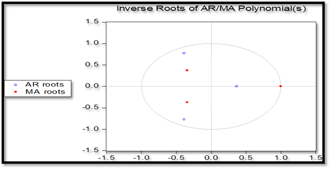
Figure 4

As illustrated in the figure above, the ARIMA (3, 1, 3) model is stable as the corresponding inverse roots of the characteristic polynomial lie in the unit circle.

5.0 FINDINGS

5.1 Descriptive Statistics

Table 11

Description	Statistic
Mean	2579.3
Median	2166.5
Minimum	58
Maximum	7646
Standard deviation	2453.9
Skewness	0.71616
Excess kurtosis	-0.77802

The mean GDP per capita is positive, i.e 270.07 USD. The minimum GDP per capita is 58 USD while the maximum is 7646 USD. Skewness is 0.71616 and it is positive, indicating that the Botswana GDP per capita data is positively skewed and non-symmetric. Kurtosis has been found to be -0.77802, meaning that the Y series is indeed not normally distributed.

5.2 Results Presentation[1]

Table 12

ARIMA (3, 1, 3) Model: P: (0.37) (0.16) (0.00) (0.02) (0.19) (0.00) S. E: (0.17) (0.23) (0.14) (0.27) (0.43) (0.29)
Variable	Coefficient	Standard Error	Z	p-value
AR (1)	-0.152563	0.170204	-0.8964	0.3701
AR (2)	0.319827	0.227948	1.403	0.1606
AR (3)	0.810511	0.135910	5.964	0.0000***
MA (1)	0.598088	0.266869	2.241	0.0250**
MA (2)	-0.568689	0.429988	-1.323	0.1860
MA (3)	-0.879090	0.294077	-2.989	0.0028***

Interpretation of Results

The AR (3) coefficient is positive and statistically significant at 1% of level of significance This indicates the importance of previous lags of GDP per capita for up to 3 years back. The MA (1) coefficient is positive and statistically significant at 5% level of significance while the MA (3) coefficient is negative and statistically significant at 1% level of significance. The significant coefficients of the moving average terms point to the relevance of previous period shocks to GDP per capita in Botswana.

Forecast Graph

Figure 5

Predicted GDP per capita (for selected years)

Figure 6

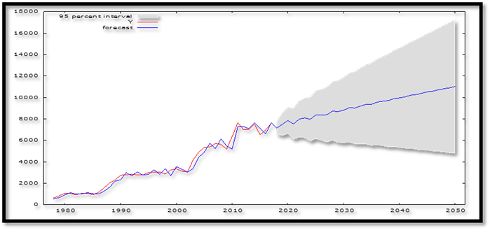
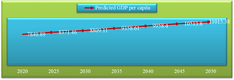
As portrayed in figures 5 and 6, Botswana is now an upper middle income country, with a projected GDP per capita of approximately 8809.11 USD by 2030. Botswana’s GDP per capita is on an upwards trajectory which is expected to continue for at least 10 years. This clearly proves beyond any reasonable doubt that the Batswana living standards will be greatly improved and poverty levels are set to tumble low minimal levels with the next decade. Indeed, Botswana; is an “African Success Story”, which can be emulated by other African countries. It is important to note that a number of factors have resulted in such a success story of Batswana. These include non-other-than good governance, political stability and prudent macroeconomic management.

6.0 POLICY RECOMMENDATIONS

i. The government of Botswana should maintain the existing political stability and good governance, something which most African countries always fail to do.

ii. Botswana monetary authorities should continue implementing the crawling peg exchange rate with preset basket weights because it has indeed served the country well.

iii. The government of Botswana should continue working tirelessly to remove barriers to private sector – led growth I order to increase the government revenue pool.

iv. The country should use the rich diamond reserves to diversify their economy.

7.0 CONCLUSION

Economic growth is always the priority of any credible government around the globe (Adebayo, 2016) and in the case of Botswana, successive governments have proved to be credible by being able to conduct good governance and seriously prioritizing economic growth and price stability ahead of selfish and politically motivated objectives. The continued increase in GDP per capita in Botswana is clear testimony that Botswana is indeed an “African Success Story” and is a good example of an African nation where rule of law is a reality and corruption is an enemy of the society. The results of this research are envisaged to help Botswana policy makers in planning for an even brighter future for Batswana.

8.0 REFERENCES

1. Adebayo, A. G (2016). Forecasting the Gross Domestic Product in Nigeria using time series analysis and a sample frame of 1960 – 2015, Journal of Business and African Economy, 2 (2): 1 – 14.

2. Asteriou, D. & Hall, S. G. (2007). Applied Econometrics: a modern approach, Revised Edition, Palgrave MacMillan, New York.

3. Barhoumi, K., Darne, O., Ferrara, L., & Pluyaud, B (2011). Monthly GDP forecasting using bridge models: application for the French economy, Bulletin of Economic Research, 1 – 18.

4. Bipasha, M & Bani, C (2012). Forecasting GDP growth rates of India: an empirical study, International Journal of Economics and Management Sciences, 1 (9): 52 – 58.

5. Dritsaki, C (2015). Forecasting real GDP rate through econometric models: an empirical study from Greece, Journal of International Business and Economics, 3 (1): 13 – 19.

6. Du Preez, J. & Witt, S. F. (2003). Univariate and multivariate time series forecasting: An application to tourism demand, International Journal of Forecasting, 19: 435 – 451.

7. Goh, C. & Law, R. (2002). Modeling and forecasting tourism demand for arrivals with stochastic non-stationary seasonality and intervention, Tourism Management, 23: 499 – 510.

8. Honde, G. J & Abraha, F. G (2015). Botswana Economic Outlook – Botswana, AfDB.

9. International Monetary Fund (2017). Botswana Staff Report for the 2017 Article IV consultation, IMF, Washington DC.

10. Junoh, M. Z. H. J (2004). Predicting GDP growth in Malaysia using knowledge-based indicators: a comparison between Neural Network and econometric approaches, Sunway College Journal, 1: 39 – 50.

11. Lu, Y (2009). Modeling and forecasting China’s GDP data with time series models, Department of Economics and Society, Hogskolan Dalarna.

12. Maipose, G.S and Matsheka, T.C (2009). The Indigenous Development State and Growth in Botswana. Chapter 5. Volume 2: 01-66

13. Nyoni, T & Bonga, W. G (2017f). An Empirical Analysis of the Determinants of Private Investment in Zimbabwe, DRJ – Journal of Economics and Finance, 2 (4): 38 – 54.

14. Nyoni, T & Bonga, W. G (2018a). What Determines Economic Growth In Nigeria? DRJ – Journal of Business and Management, 1 (1): 37 – 47.

15. Nyoni, T (2018n). Modeling and Forecasting Inflation in Kenya: Recent Insights from ARIMA and GARCH analysis, Dimorian Review, 5 (6): 16 – 40.

16. Nyoni, T. (2018i). Box – Jenkins ARIMA Approach to Predicting net FDI inflows in Zimbabwe, Munich University Library – Munich Personal RePEc Archive (MPRA), Paper No. 87737.

17. Okasha, M.K and Yaseen, A.A (2013). Comparison Between Arima Models And Artificial Neural Networks In Forecasting Al-Quds Indices Of Palestine Stock Exchange Market. Conference paper. Research Gate.

18. Onuoha, D. O., Ibe, A., Njoku, C., & Onuoha, J. I (2015). Analysis of the Gross Domestic Product (GDP) of Nigeria: 1960 – 2012, West African Journal of Industrial & Academic Research, 14 (1): 81 – 90.

19. Song, H., Witt, S. F. & Jensen, T. C. (2003b). Tourism forecasting: accuracy of alternative econometric models, International Journal of Forecasting, 19: 123 – 141.

20. Wabomba, M. S., Mutwiri, M. P., & Mungai, F (2016). Modeling and forecasting Kenyan GDP using Autoregressive Integrated Moving Average (ARIMA) models, Science Publishing Group – Science Journal of Applied Mathematics and Statistics, 4 (2): 64 – 73.

Cite this Article: Nyoni, T; Muchingami, L; Olebogeng M; Joe J; Georgina M (2021). Modeling and Forecasting Botswana’s Growth Domestic Product (GDP) per Capita. Greener Journal of Economics and Accountancy, 9(1):1-9,

---

[1] The *, ** and *** means significant at 10%, 5% and 1% levels of significance; respectively.