Highlighting the Fine Structure of the Seismic Zones
of the Western Branch of the East African Rift System Using the Unified Characterization
Scale and Its Geological Implication.
Previous research aimed at
characterizing the seismicity of the DRC and its surroundings (Mukange, 2016; Mukange, 2021b)
revealed that the seismic activity of the DRC is subdivided into two large
zones: a non-rift zone (10°E -25°E) of low seismicity and a rift zone
(25°E-35°E) of high seismicity; the average degree of heterogeneity of the
region is 60%, with seismic activity concentrated in the main faults.
The main objective of this work is to highlight the fine structure of the
Rift zones using the model which exploits the notion of seismic species and
the precise location of the main underground faults by positing the
hypothesis that: “the main faults are located in places where the module of
seismic activity is at its peak”. We are interested in the rift zone
(30°E-35°E. 6°N-14¨S). This zone includes the square grid zones A41, A42,
A42, A44, A51, A52, A52 and A54 with a side of 5° each. The demonstration of
their fine structure consists of subdividing them into squares of side 1°
each by calculating certain parameters deduced from the fundamental seismic
parameters covering the period from 1975 to 2013. This model, introducing new
concepts, led to the results following, some of which go beyond the known:
Regarding the fine structure, we note:
·that the rift zone (25-35°E), formerly homogeneous, is now subdivided
into two distinct sub-zones:
·The area located between 25 and 30°E (A42, A43 and A44). However, we notethat the structure of zone A44 (Upemba
rift zone in the upper Katanga region) straddles between A42T (Virunga-Lake Kivu zone) and A43T (Tanganyika zone).
·The zone between 30 and 35°E (A51, A52, A53 and A54). However, zones
A42T (Kivu zone) and A54T (Malawi zone) have some similarities,
·The rate of resemblance between the two sub-zones is 25%: the first
zone is less seismic than the second, one having a form factor (III), the
other (IV),
·that the structure of the entire
established DRC is almost identical to that of the A42B'' zone (Virunga zone at a depth exceeding 30km).
The exploitation of the
aforementioned hypothesis and our model made it possible to locate the main
escaped faults and to note that:
·These faults are exactly located in areas with intense seismic
activity; going deeper, these faults change position: the shape is no longer
vertical or rectilinear, but wavy and serpentine.
·from the surface to a depth of 20 km, the faults ofKivu (A42) and Tanganyika (A43) zones are
located near the rift, to move away from it beyond the depth of 20 km
(corresponding to the position average of the Conrad discontinuity),
·While the position of the main faults at layer G (0-10 km) is located
at A5 for seismic zone A42, these faults are located at zone A3 for A43 for
the same layer (G) and the opposite at the layer C (10-20 km) and are all
located at A1 beyond 20 km.
Accepted:06/12/2023
Published: 30/12/2023
*Corresponding
Author
Prof. MukangeBesaAnscaire
E-mail: anscairbesa@ yahoo.fr
Keywords: fine
structure, East African rift, Congolese Rift, seismic species,
characterization scale, heterogeneity rate, resemblance rate, fault
location, d-value
1. INTRODUCTION
The map in figure (2) from previous studies (Mukange, 2016; Mukange, 2021a,b) carried out on the characterization of the seismicity of
the DRC and its surroundings reveals that:
vSeismic activity in the DRC is subdivided
into two large zones:
vA non-rift zone (10°E-25°E) characterized
by low seismicity,
vA rift zone (25°E-35°E) of high
seismicity,
vA degree of heterogeneity of 65% and 55%
following respectively the horizontal and vertical subdivision, i.e. an average
degree of heterogeneity of 60%,
vEach grid zone (square with side 5°) has a
degree of heterogeneity of 0%, i.e. homogeneous at 100%.
vSeismic activity is concentrated in the
main faults,
The main objective of this work is to highlight the
fine structure of the Rift zones. To do this, thanks to the design of the
unified characterization scale based on the notion of seismic species, it will
be necessary, on the one hand, to calculate the following parameters: the rate
or degree of heterogeneity of the grid zones, their rate resemblance and
conservation of seismic species and on the other hand, to precisely locate the
main underground faults by positing the hypothesis that: "the main faults
are located in places where the module of seismic activity is at paroxysm.” The
judicious exploitation of these parameters would allow better monitoring of
geological phenomena and geodynamics, with an opening towards indirect
geological prospecting.
The East African Rift System appears as a continental
extension of the global system of lithospheric fractures which wind through the
middle of the Atlantic and Indian Oceans and which extend into the eastern part
of the African Continent via the Gulf of Aden and the Red Sea ( Mukange, 2016; Boden et al. 1988; Bantidi,
2014a). This system of fractures is made up of two branches, namely:
vThe eastern branch which, from the Afar
triangle, crosses Ethiopia and Kenya to the northern Tanzanian divergence
(Figure 1a); Mukange, 2012).
vThe western branch is made up of a system
of fractures which cross the garland of the Great Lakes, that is to say, from
Lake Albert (617 m altitude) passes through Lakes Edouard
(912m), Kivu (1462m), Tanganyika (780m), Rukwa
(782m), Malawi (460m) and continues south to Mount Beira in Mozambique and
southwest to Lake Kariba, Zimbabwe. This branch
therefore covers most of the eastern provinces of the DRC from latitude 4°N to
latitude 8°S. From the Red Sea to the Zambezi the East African Rifts cover more
than 6000km long and 40 to 60km wide. The two branches split in two at the
level of the Aswan lineament and join at the level of Lake Malawi (Figure 1a).
The seismic activity of the DRC also includes that
characteristic of intra-plate fractures which thus affects the entire Congolese
basin known as the “Congolese craton”.
Figure 1a: The East African rift system (Mavonga,
2009)
Fig. 1b: Distribution of epicenters in the DRC (1972-2008)
2. DATA AND METHOD OF ANALYSIS
This point is presented in two sub-points:
2.1. Analysis data
We analyze data collected through various sources (www.usgs.organd
www.isc.ac.uk), covering the period from 1975 to 2013 over the geographical
area between 6° North and 14° South latitude and between 25° East
and 35° East longitude. This area includes the Rift grid zones A41, A42, A42,
A44, A51, A52, A52 and A54 (figures 1b-2). Particular emphasis will be placed
on zones A42, A42 and A44 located in the Congolese rift (Figure 1b).
2.2 Analysis method
Achieving our objectives requires the design of the
unified characterization scale. This scale must integrate various classic
parameters that we will have to calculate in each sub-zone; these are the
following parameters:
vThe total number of earthquakes,
vThe total energy released by earthquakes,
vMaximum Magnitude,
vThe maximum depth of the hypocenters,
vSurface area of each
sub-zone,
vVolume of each subzone,
vDensity of earthquakes,
vEnergy density,
vThe b-value (Lay and al., 1995) and the
“d-value”,
vThe degree of heterogeneity of the area,
vThe rate of resemblance of species,
vThe conservation rate of species.
For explanations not provided here relating to the
calculation of certain parameters, we invite the reader to consult the
literature (Mukange, 2021a-b; Mukange
2023a-bc); this is particularly the case for the rate of heterogeneity.
Figure 2: Seismic zoning in the Democratic Republic of Congo for seismic
hazard assessment (Mukange, 2021b)
Figure 3 a:
structural signature of the seismicity of the DRC
The map results above lead to obtaining the figure
below called the structural signature of the seismic zone.
The characterization work will be carried out on each
grid zone A41, A42, A43, A44, A51, A52, A52 and A54. Particular emphasis will
be given to zones A42 and A43 due to the fact that one contains Lake Kivu in
the Virunga volcano-seismic region,
the other contains Lake Tanganyika in the Tanganyika seismic sub-zone (Mavonga, 2009; Figure 1).
The work of
characterizing the internal structure of each of these zones therefore consists
of:
vSubdivide each grid zone (Aij) according to depth (Table 3a); this slice is called
depth zone,
vSubdivide each depth zone into vertical
(Ai) and horizontal (Bj) sub-zones of one degree
width (Table 2). Since each sub-zone Aij is a square
of side 5°, by subdividing it thus, it will therefore be composed of
twenty-five square sub-zones of side 1° each,
vCalculate the aforementioned
characterization parameters in each Ai and Bj,
vSearch for seismic species in each subzone
Ai and Bj,
vAssign the seismic level and the
appropriate color to each Ai and Bj,
vCalculate the module and assign the appropriate
color to each grid zone Aij (Ai, Bj),
vDiscuss and interpret the results,
vDraw the general conclusion and
perspectives.
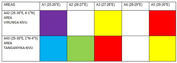
Table 1: Boundaries of the DRC rift grid
zones under study
No.
AREA
LONGITUDE
LATITUDE
1
A42
25°E-30°E
1°N-4°S
2
A43
25°E-30°E
4°S-9°S
2
A44
25°E-30°E
9°S-14°S
4
A51
30°E-35°E
6°N-1°S
5
A52
30°E-35°E
1°N-4°S
6
A53
30°E-35°E
4°S-9°S
7
A54
30°E-35°E
9°S-14°S
Table 2: Subdivision of zones (Aij) into vertical (Ai)
and horizontal (Bj) sub-zones
ZONE A42 (25°E-30°E;
1°N-4°S)
No.
ZONES Ai and Bj
LONGITUDE
LATITUDE
01
A1
25°E-26°E
1°N-4°S
02
A2
26°E-27°E
1°N-4°S
02
A3
27°E-28°E
1°N-4°S
04
A4
28°E-29°E
1°N-4°S
05
A5
29°E-20°E
1°N-4°S
06
B1
1°N-0°N(S)
25°E-20°E
07
B2
0°-1°S
25°E-20°E
08
B3
1°S-2°S
25°E-20°E
09
B4
2°S-2°S
25°E-20°E
10
B5
2°S-4°S
25°E-20°E
Table 3: Subdivision of zones (Aij) into depth zones for A42 and A43
GRID AREA A42 AND A43
No.
ZONE-DEPTH
DEPTH SECTION (km)
1
A42G
A43G
[0-10]
2
A42B
A43B
] 10-20]
2
A42B'
A43B'
] 20-20]
4
A42B''
A43B''
>20
5
A42C
A43C
] 0-20]
6
A42C'
A43C'
] 20-40]
7
A42C''
A43C''
>40
3. PRESENTATION AND
DISCUSSION OF RESULTS
3.1.Presentation of the results
The values of the various calculated
parameters are contained, for illustrative purposes for zone A42, in the table
below
Table 4:Illustration
of the parameters calculated in each sub-zone of zone Aij,
case of A42
Below-
Areas
b-value
λb-value
d-value
λd-value
Number (%)
Energy (%)
Magnitude
maximum
Max hypocenter (km)
Volume density of earthquakes (%)
Energy volume density(%)
A1
0.669
1,541
0.0224
0.076
2.2
1.2
6.1
40
2.2
1.2
A2
1.0912
2,514
0.0126
0.021
8.2
0.1
5.4
96
17.0
0.2
At 3
0.9179
2,115
0.0492
0.112
9.4
20.8
5.5
25
52.6
119.0
A4
0.8262
1,904
0.046
0.105
11.2
12.0
6.4
40
56.2
65.1
AT 5
0.9706
2,226
0.0487
0.111
68.0
64.6
6.7
168
81.0
76.9
B1
0.999
2,202
0.045
0.102
27.9
10.4
6.2
168
45.2
12.4
B2
1.0526
2,425
0.046
0.105
14.6
0.2
5.5
85
24.2
0.6
B3
0.8865
2,042
0.0522
0.119
17.0
17.7
6.5
40
84.9
88.5
B4
0.9505
2,190
0.0477
0.108
14.8
9.4
6.4
46
64.2
40.8
B5
0.8227
1,919
0.024
0.055
15.8
41.7
6.7
96
22.8
86.8
3.2. Discussion of results
The discussion of the results is carried out in two
main stages: the design of the unified characterization scale leading to the
attribution of a seismic species to each sub-zone and the discussion itself
(interpretation).
3.2.1. Design of the characterization scale
The characterization of the seismic activity of an
area involves the design of a unified characterization scale which can
reasonably integrate all the calculated parameters (Table 4). For this purpose,
a characterization scale is developed consisting of five parameters and defined
as follows:
X is the “form factor” which can take the value O, I,
II, III, IV or V, with:
v0 if the area is aseismic,
vI if the maximum magnitude recorded is
between,
vII if the maximum magnitude recorded is
between,
vIII if the maximum recorded magnitude is
between,
vIV if the maximum recorded magnitude is
between,
vV if the maximum magnitude recorded is
between,
The group of numbers (1; 2; 3; 4) in subscript
constitutes the “structure factor”, defined as follows:
the number 1 relates
to the volume density of the seismic energy released in each sub-zone:
vif this density is ≤ 50%, then the
number 1 takes the index “a”,
vif this density is between 50% and 100%,
then the number 1 takes the index “b”,
vif this density is greater than 100%, then
the number 1 takes the index “c”,
the number 2 relates
to the volume density of the number of earthquakes in each sub-zone:
vif this density is ≤ 50%, then the
number 2 takes the index “a”,
vif this density is between 50% and 100%,
then the number 2 takes the index “b”,
vif this density is > 100%, then the
number 2 takes the index “c”,
The number 3 relates to the λb-value parameter:
vIf λb-value >2, then it takes the index
“a”,
vIf 1< λb-value≤
2, then it takes the index “b”,
vIf λb-value <1, then it takes the index
“c”,
Note that λb-value = 2.204 b-value. This parameter measures
seismic activity.
The number 4 relates to the λd-value parameter:
vIf the λd-value
>0.2, then it takes the index “a”,
vIf the 0.1< λd-value≤
0.2, then it takes the index “b”,
vIf the λd-value
<0.1, then it takes the index “c”,
Note that λd-value = 2.272d-value. This parameter is related to
the structure of the soil.
3.2.2. Presentation of seismic species
The application of this scale to the various zones
generates seismic species and levels (Tables 5-10). The seismic level is next
to each seismic species. This scale also contains the
seismic species discovered in the USA and Indonesia zone.
Table 5: Presentation of species and seismic level of each sub-zone
AREA DRC A42T
SEISMIC SPECIES
DRC ZONE A43T
SEISMIC SPECIES
DRC ZONE A44T
SEISMIC SPECIES
ZONE DRC A51T
SEISMIC SPECIES
A1
IIIaabc
43
A1
IIabac
28
A1
IICCab
40
A1
IIIbbbC
61
A2
IIaaac
20
A2
IIaaaC
20
A2
IICabC
36
A2
IIIbCbC
65
A3
IIcbab
37
A3
IIIabbC
49
A3
IICbbC
38
A3
IVbCbC
82
A4
IIIbbbb
60
A4
IIabac
28
A4
IIabaC
28
A4
IaabC
4
A5
IIIbbab
59
A5
IIIccbb
75
A5
IIabaC
28
A5
IaabC
4
B1
IIIaaab
42
B1
IIaCab
22
B1
IICCaC
41
B1
IIIccbc
76
B2
IIaaab
18
B2
IIIccbb
75
B2
IIabbC
20
B2
IIIccbc
76
B3
IIIbbab
59
B2
IIIaCbb
52
B3
IICCab
40
B3
IVccab
82
B4
IIIabab
46
B4
IIIaCbb
52
B4
IICCaa
39
B4
IIabaC
28
B5
IIIbabc
56
B5
IIIaabC
44
B5
IIabaC
28
B5
IIabaC
28
Table 6: Presentation of species and seismic level of each sub-zone
(continued)
ZONE DRC A42B
SEISMIC SPECIES
ZONE DRC A42B'
SEISMIC SPECIES
ZONE DRC A42B''
SEISMIC SPECIES
ZONE GROUND A43C''
SPECIES
A1
IIaaaa
17
A1
IIaacb
25
A1
IIIcbbc
72
A1
0
0
A2
Iaaca
5
A2
IIaacb
25
A2
IIaabc
22
A2
0
0
A3
IIaaca
24
A3
IIaabb
22
A3
Iabbc
11
A3
0
0
A4
IIIbaba
55
A4
IIaaab
19
A4
IIacbc
25
A4
Iccbc
15
A5
IIIabba
47
A5
IIaabb
22
A5
IIIccac
75
A5
0
0
B1
IIIaaba
42
B1
IIaabb
22
B1
IIIccac
75
B1
0
0
B2
IIaaba
21
B2
IIaabb
22
B2
IIabbc
20
B2
Icccc
16
B3
IIIbaba
55
B3
IIaabb
22
B3
Iacac
12
B3
0
0
B4
IIaaba
21
B4
IIaabb
22
B4
IIIccbc
77
B4
Iaabc
4
B5
Yaaaa
1
B5
IIaaab
18
B5
IIaabc
22
B5
0
0
Table 7: Presentation of species and seismic level of each sub-zone
(continued)
ZONE DRC A43B
SEISMIC SPECIES
ZONE DRC A43B'
SEISMIC SPECIES
ZONE DRC A43B''
SEISMIC SPECIES
ZONE DRC A42C
SEISMIC SPECIES
A1
0aaaa
0
A1
0aaaa
0
A1
Iacba
14
A1
Iabaa
7
A2
Yaaaa
1
A2
Iaaba
3
A2
Iabba
9
A2
Yaaaa
1
A3
IIIbaca
58
A3
Iaaba
3
A3
Iabba
9
A3
Iabaa
7
A4
Iaaaa
1
A4
Iabba
9
A4
Iabbc
11
A4
IIIccaa
75
A5
IIIabba
48
A5
IIIbbca
65
A5
IIIacba
52
A5
IIIccaa
75
B1
IIaaba
21
B1
Iaaba
3
B1
IIabba
29
B1
IIIbcaa
66
B2
IIIaaca
46
B2
IIbbca
65
B2
IIacab
33
B2
IIabaa
26
B3
IIaaca
24
B3
IIaaca
24
B3
Iacab
13
B3
IIIcbaa
71
B4
IIaaca
24
B4
Iaaba
3
B4
IIIccca
80
B4
IIIbbaa
60
B5
IIIbaca
58
B5
Iaaba
3
B5
IIaaba
21
B5
IIIcbba
73
Table 8: Presentation of species and seismic level of each sub-zone
(continued)
DRC ZONE A52T
SEISMIC SPECIES
ZONE DRC A53T
SEISMIC SPECIES
ZONE DRC A54T
SEISMIC SPECIES
ZONE DRC A42G
SEISMIC SPECIES
A1
IIaCaC
22
A1
Ivbcbc
82
A1
IIabac
28
A1
IIaaac
20
A2
IIIcbbc
71
A2
IIIacbc
52
A2
IIIacbc
52
A2
IIaaac
20
A3
Iaaac
2
A3
Ivabbc
80
A3
IIabbc
20
A3
IIabac
28
A4
IIIccac
74
A4
IIaaac
20
A4
IIIacac
50
A4
IIIccbc
76
A5
IIaCaC
22
A5
IIIacbc
52
A5
IVccbc
84
A5
IIIbcac
64
B1
IIIcbbc
71
B1
IIacac
22
B1
IIIabbc
49
B1
IIIacac
50
B2
IIabac
28
B2
IVaabc
79
B2
IVccbc
84
B2
IIabac
28
B3
IIabac
28
B3
IIIacac
50
B3
IVccbc
84
B3
IIIcbac
69
B4
IIabac
28
B4
IVacbc
81
B4
IIacac
22
B4
IIIbbac
59
B5
IIIccac
74
B5
IIIabbc
49
B5
IIIacbc
52
B5
IIIcbbc
72
Table 9: Presentation of species and seismic level of each sub-zone
(continued)
ZONE DRC A42C'
SEISMIC SPECIES
ZONE GROUND A42C''
SEISMIC SPECIES
ZONE DRC A43G
SEISMIC SPECIES
ZONE DRC A43C
SEISMIC SPECIES
A1
IIIcabb
70
A1
Yaaaa
1
A1
IIaaac
20
A1
IIabac
28
A2
IIaabc
23
A2
0aaaa
0
A2
IIaaac
20
A2
IIaaab
19
A3
IIaabb
22
A3
0aaaa
0
A3
IIIbabc
56
A3
IIIcbba
72
A4
IIacab
33
A4
Iabbc
11
A4
IIaaac
20
A4
IIacaa
22
A5
IIIccab
76
A5
IIccbc
43
A5
IIIaaac
43
A5
IIIccaa
75
B1
IIIccab
76
B1
IIccbc
43
B1
IIaaac
20
B1
IIabab
27
B2
IIabbb
30
B2
IIaabc
23
B2
IIaabc
23
B2
IIIcbaa
71
B3
IIabbb
30
B3
IaDabc
4
B3
IIIbaac
55
B3
IIIccaa
75
B4
IIIabbb
50
B4
Iacbc
15
B4
IIaaac
20
B4
IIabaa
26
B5
IIabab
27
B5
Iaabc
4
B5
IIaaac
20
B5
IIIcbaa
71
Table 10: Presentation of seismic species and level of each sub-zone (end)
ZONE A43C'
A1
A2
A3
A4
A5
SEISMIC SPECIES
Iabbc
11
Iabbc
11
Iabbc
11
Iabab
8
IIIccbb
78
ZONE A43C'
B1
B2
B3
B4
B5
SEISMIC SPECIES
IIacbb
35
IIIcccb
81
IIabbc
31
IIIabbb
50
IIabbb
30
3.2.3. Calculation of the similarity
rate
The rate of resemblance between two zones is done by
comparing the respective seismic species or by setting a species taken as a
unit of measurement (reference). The calculation is carried out as follows:
The
characterization scale, giving rise to a seismic species, is written X1224. Let
zones A and B have respective seismic species XA1A2A2A4A and XB1B2B2B4B. The
resemblance rate is calculated based on the form factor (X) and the structure
factor (1, 2, 3.4) using the following formula:
Form factor
vIf ,𝑋𝐴 − 𝑋𝐵 = 0, then the resemblance
rate is 50%,
vIf ,𝑋𝐴 − 𝑋𝐵 = 1, then the resemblance
rate is 40%,
vIf ,𝑋𝐴 − 𝑋𝐵 = 2 then the resemblance
rate is 30%,
vIf ,𝑋𝐴 − 𝑋𝐵 = 3, then the resemblance
rate is 20%,
vIf ,𝑋𝐴 − 𝑋𝐵 = 4 , then the resemblance
rate is 10%,
vIf ,𝑋𝐴 − 𝑋𝐵 = 5 , then the resemblance
rate is 0%,
Structure factor
vIf , 1𝐴 = 1𝐵 , then the resemblance
rate is 15%, otherwise 0%
vIf , 2𝐴= 2𝐵
, then the resemblance rate
is 15%, otherwise 0%
vIf , 3𝐴 = 3𝐵 , then the resemblance
rate is 10%, otherwise 0%
vIf , 4𝐴 = 4𝐵 , then the resemblance
rate is 10%, otherwise 0%
We see that the total is 100%.
Example: calculate the rate of resemblance between the
zones characterized by the following species IVccba
and Icbbc then calculate it by taking the species IVcccc as a unit of measurement (reference). The first rate
is called the relative resemblance rate, the other is
the absolute resemblance rate.
Example of calculating the relative similarity rate
Form
factor
vIVA − IB = 2, then the resemblance rate is 20%,
Structure factor
vLike 1A(c) = 1B(c) ,then the resemblance
rate is 15%,
vLike 2A(c) ≠ 2B(b) ,then the resemblance
rate is 0%,
vLike 3A(b) = 3B (b) ,then the resemblance
rate is 10%,
vLike 4A(a) ≠ 4B(c) ,then the resemblance
rate is 0%,
The total similarity rate is 45% (20%+15%+0%+10%+0%)
Example of calculating the absolute resemblance rate
(we leave the task to the reader)
3.2.4. Results interpretation
The interpretation of the results focuses on the
parameters below.
3.2.4.1. Seismic species, seismic levels and color
Observation of the results of tables (5-10) shows
that:
vIn total, we identified 89 distinct
seismic species,
vThere are 28 (42%) seismic species common
to all areas,
vThere are 17% of species exclusive to
zones A51, A52, A52 and A54, zones between 30 and 35°E,
vThere are 17% of seismic species exclusive
to zone A42, subdivided into depth zones (A42G, A42B, A42B', A42B'', A42C,
A42C', A42C'') according to table (3),
vThere are 17% of species exclusive to zone
A43, also subdivided into depth zones (A43G, A43B, A43B', A43B'', A43C, A43C',
A43C'').
The statistics indicate:
vThe first zone (A4j) is less seismic than
the second (A5j): one having a form factor (III), the other (IV); As a result,
we see that their intersection is empty (figure 3b),
vThe resemblance rate, based on structural
factors, between these two zones is 17%: there is one common element out of a
total of six (Figure 3c),
vThe structure of the DRC (25°-30°E) is
more stable than that of Malawi-Zambezi (30°E-35°E),
Figure 3b: comparison of seismic species between the two zones of the A4j
rift (25°E-30°E) and A5d (30°E-35°E)
Figure 3c: comparison of the structure factors between the two zones of the
A4j rift (25°E-30°E) and A5d (30°E-35°E)
3.2.4.2. Seismic zoning of grid zones
The notion of grid zones (Aij)
is related to that of vector representation (Mukange,
2021a-b)
The module (c) of each subzone Cij
is calculated using the formula (2.12)
Or, and correspond respectively to the seismic levels
of the vertical subzones (Ai) and (Bj) contained in
tables (5-10).
Table 11: Color code
relating to module slice and quantum level
MODULE (c)
QUANTUM LEVEL
COLORS
0
BLACK
1
PURPLE
2
LIGHT BLUE
3
DARK BLUE
4
LIGHT GREEN
5
DARK GREEN
6
YELLOW
7
ORANGE
8
LIGHT RED
9
DARK RED
The application of this code to each zone, and for illustration purposes to zone A42, leads to
the results contained in the Table below.
Table 12: Illustration of the results
from the previous table for the A42T zone
Area
DRC A42T
Seismiclevel of Ai
Seismiclevel of Bi
Module of Aij (Ai,Bj)
Quantum level
Color code
Colorstatistics
A11
42
42
60
4
LIGHT GREEN
28%
A12
42
18
47
4
LIGHT GREEN
28%
A13
42
59
72
5
DARK GREEN
44%
A14
42
46
62
5
DARK GREEN
44%
A15
42
56
71
5
DARK GREEN
44%
A21
20
42
47
4
LIGHT GREEN
4%
A22
20
18
27
2
LIGHT BLUE
4%
A23
20
59
62
5
DARK GREEN
44%
A24
20
46
50
4
LIGHT GREEN
4%
A25
20
56
59
4
LIGHT GREEN
4%
A31
27
42
56
4
LIGHT GREEN
4%
A32
27
18
41
3
PURPLE
4%
A33
27
59
70
5
DARK GREEN
44%
A34
27
46
59
4
LIGHT GREEN
4%
A35
27
56
67
5
DARK GREEN
44%
A41
60
42
72
5
DARK GREEN
44%
A42
60
18
62
5
DARK GREEN
44%
A43
60
59
84
6
YELLOW
20%
A44
60
46
76
6
YELLOW
20%
A45
60
56
82
6
YELLOW
20%
A51
59
42
72
5
DARK GREEN
44%
A52
59
18
62
5
DARK GREEN
44%
A53
59
59
82
6
YELLOW
20%
A54
59
46
75
5
DARK GREEN
44%
A55
59
56
81
6
YELLOW
20%
The results in the table above and others in the
appendix lead to the highlighting of zoning maps, representing the chromatic
structure of seismic zones.
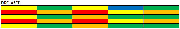
NB: Each sub-zone delimited by color is a square with
a side of one degree (1°).
Figure 4a: Seismic
zoning map of the DRC A42T zone
Figure 4b: Seismic
zoning map of the DRC A43T zone
Figure 4c: Seismic zoning map of the DRC A44T zone
Figure 4d: Seismic zoning map of the DRC A51T zone
Figure 4e: Seismic
zoning map of the DRC A52T zone
Figure 4f: Seismic
zoning map of the DRC A53T zone
Figure 4g: Seismic
zoning map of the DRC A54T zone
Figure 4h: Seismic
zoning map of the DRC A42G zone
Figure 4i: Seismic
zoning map of the DRC A42B zone
Figure 4j: Seismic
zoning map of the DRC A42B' zone
Figure 4k: Seismic
zoning map of the DRC A42B'' zone
Figure 4l: Seismic
zoning map of the DRC A42C zone
Figure 4m: Seismic
zoning map of the DRC A42C' zone
Figure 4n: Seismic
zoning map of the DRC A42C zone
Figure 4o: Seismic
zoning map of the DRC A43 G zone
Figure 4p: Seismic
zoning map of the DRC A43B zone
Figure 4q: Seismic
zoning map of the DRC A43B' zone
Figure 4r: Seismic
zoning map of the DRC A43B'' zone
Figure 4s: Seismic
zoning map of the DRC A43C zone
Figure 4t: Seismic zoning map of the DRC A43C' zone
Figure 4u: Seismic zoning map of the DRC A43C' zone
Depending on the color arrangements, we observe that
all these 21 zones are grouped into two shapes:
·A symmetrical
shape of the colors in relation to zone A3; these are zones A51T, A52T, A53T
and A54T located between 30° and 35°E,
·A bipolar form
(two groups of colors) for all areas located between 25° and 20°E; these are
the A42T, A43T, A44T and their derivatives.
3.2.4.3. Calculation of the degree of heterogeneity and the rate of
resemblance
The degree or rate of heterogeneity is calculated by
taking the ratio, as a percentage, of the total number of colors identified in
the area to ten colors retained in the color code (Figures 4). The resemblance
rate is calculated according to the formula indicated in point (2.2.2).
However, we distinguish two similarity rates (TR):
·The first,
called absolute (TR1): this is the resemblance between the maximum seismic
species taken as a reference and the maximum species observed among the Ai and Bj of the zone where we want to evaluate the rate (Tables
5-10 ; Tables 13-14),
·The second,
called relative (TR2) or cumulative calculated according to the depth of the
layers going from the surface downwards (Tables 15-16).
Table 13: Calculation of the absolute resemblance rate for A42 zones
No.
AREAS TO COMPARE
RESEMBLANCE RATE (TR1)
0
A42T-A42T
100%
1
A42T-A42G
60%
2
A42T-A42B
75%
3
A42T-A42B'
50%
4
A42T-A42B''
60%
5
A42T-A42C
50%
6
A42T-A42 C'
60%
7
A42T-A42 C''
50%
Table 14: Calculation of the absolute resemblance rate for A43 zones
No.
AREAS TO COMPARE
RESEMBLANCE RATE (TR1)
0
A43T-A43T
100%
1
A43T-A43G
60%
2
A43T-A43B
50%
3
A43T-A43B'
50%
4
A43T-A43B''
80%
5
A43T-A43C
80%
6
A43T-A43 C'
90%
7
A43T-A43 C''
60%
Table 15: Calculation of the relative similarity rate for A42 zones
No.
AREAS TO COMPARE
RESEMBLANCE RATE (TR2)
0
A42T-A42T
100%
1
A42T-A42G
60%
2
A42G-A42B
60%
3
A42B-A42B'
55%
4
A42B'-A42B''
40%
5
A42B''-A42C
80%
6
A42C-A42 C'
90%
7
A42C'-A42 C''
80%
Table 16: Calculation of the relative similarity rate for A43 zones
No.
AREAS TO COMPARE
RESEMBLANCE RATE (TR2)
0
A43T-A43T
100%
1
A43T-A43G
60%
2
A43G-A43B
65%
3
A43B-A43B'
85%
4
A43B'-A43B''
60%
5
A43B''-A43C
90%
6
A43C-A43C'
80%
7
A43C'-A43 C''
70%
The figure below shows the distribution of similarity
and heterogeneity rates for each zone.
Figure 5: Distribution of the absolute heterogeneity and resemblance rate
according to the zones
Figure 6a: Distribution of absolute (TR1) and relative (TR2) resemblance
rates according to zones A42 and A43
From these curves, the following observations emerge:
·With a few
exceptions, there is a correlation between the absolute resemblance rate (TR1)
and the relative resemblance rate (TR2), (Figure 6);
·With a few
exceptions, except at A42G and A42B, there is a correlation between the
absolute or relative rate of resemblance and the rate of heterogeneity (Figure
5);
·There is a
correlation between the number of curves and the rate of heterogeneity; in
fact, we see that the number of curves decreases with the rate of
heterogeneity: at less than 50% of this rate, there are at most three
structural curves (Figure 5 and Figures 7).
·As a result,
another heterogeneity rate can be calculated based on the number of visible
curves (out of five in total) on the structural curves (geo-seismic signature,
figures 7a-l)
Figure 6b: Heterogeneity rate calculated based on geo-seismic signatures
The figure above groups the zones into four classes,
made up of zones with a rate of 40%, 50%; 60% and 70% whose distribution of
zones is represented by the graph below.
Figure 6c: Weight of each class made up of zones according to the level of
heterogeneity rate of geoseismic signatures
We see that classes (1 and 3, odd) are dominant; they
cover 76% of the areas
3.2.4.3. Species conservation rate
Calculating the conservation rate of species (Tables
17-20), inverse of the disappearance rate, consists of comparing the common
species between two zones. Each zone has, at most, ten seismic species (Tables
5-10)
Table 17: Calculation of the absolute conservation rate of the species for
A42 zones
No.
AREAS TO COMPARE
CONSERVED SPECIES
CONSERVATION RATE
DISAPPEARANCE RATE
1
A42T-A42G
IIaaac
10%
90%
2
A42T-A42B
None
0%
100%
3
A42T-A42B'
IIaaab
10%
90%
4
A42T-A42B''
None
0%
100%
Table 18: Calculation of the absolute conservation rate of the species for
A43 zones
No.
AREAS TO COMPARE
CONSERVED SPECIES
CONSERVATION RATE
DISAPPEARANCE RATE
1
A43T-A43G
IIaaac
10%
90%
2
A43T-A43B
None
0%
100%
3
A43T-A43B'
None
0%
100%
4
A43T-A43B''
IIacab
10%
90%
The tables above calculate the conservation rate of
the zones step by step (relative rate)
Table 19: Calculation of the relative conservation rate of the species for
A42 zones
No.
AREAS TO COMPARE
CONSERVED SPECIES
CONSERVATION RATE
DISAPPEARANCE RATE
1
A42T-A42G
IIaaac
10%
90%
2
A42G-A42B
None
0%
100%
3
A42B-A42B'
None
0%
100%
4
A42B'-A42B''
None
0%
100%
Table 20: Calculation of the relative conservation rate of the species for
A43 zones
No.
AREAS TO COMPARE
CONSERVED SPECIES
CONSERVATION RATE
DISAPPEARANCE RATE
1
A43T-A43G
IIaaac
10%
90%
2
A43G-A43B
None
0%
100%
3
A43B-A43B'
0aaaa, IIaaca
20%
80%
4
A43B'-A43B''
Iabba
0%
100%
These tables indicate an average conservation rate of
5%, 5%, 2.5% and 5% for figures (17-20) respectively. We conclude that species
are rarely preserved as a function of depth.
3.2.4.4. Structural curve (geo-seismic signature)
The results in table (12) and others in the appendix,
in particular, have been transformed into the curves below, called “geo-seismic
signatures” or “structural signatures”. The geodynamics of an area can be
monitored based on the variation of the signature over time.
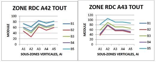
Figure 7a: Structural curves (signature) of zones A42T and A43T
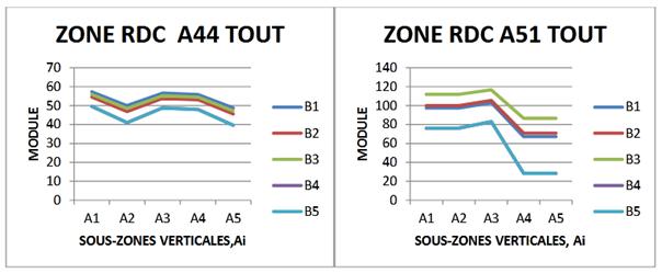
Figure 7b: Structural curves (signature) of zones A44T and A51T
Figure 7c: Structural curves (signature) of zones A52T and A53T
Figure 7d: Structural curves
(signature) of zones A54T and A42G
Figure 7e: Structural curves (signature) of zones A42B and A42B'
Figure 7f: Structural curves (signature) of zones A42B'' and A43G
Figure 7g: Structural curves (signature) of zones A43B and A43B'
Figure 7h: Structural curves (signature) of zones A43B'' and A42
Figure 7i: Structural curves (signature) of zones A42C' and A42C''
Figure 7j: Structural curves (signature) of zones A43C and A43C'
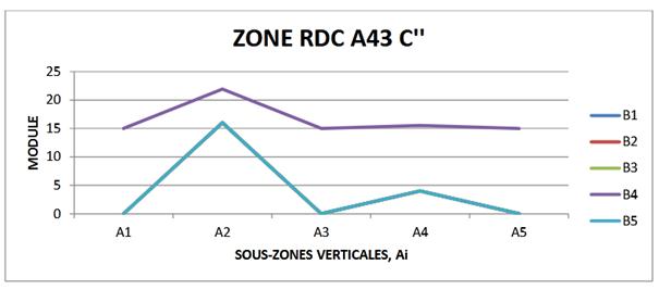
Figure 7k: Structure curves (signature) of A43C'' zones
The observation of these signatures groups them into
five modes (Table 21).
Table 21: classification of zones according to the modes or shapes of the
structural curves
-The majority (41%) of structures are in
the category of downward-facing concavity curves,
-Zones A42 (G
and C) and A52T are singularities; remember that zone A42 is located in the Virunga-Lake Kivu volcanic region and that zone A52 is to
its right (Figure 2).
3.2.4.5. Comparison of some structures
Among the structures above, there are those that
attract our attention; in fact we see that:
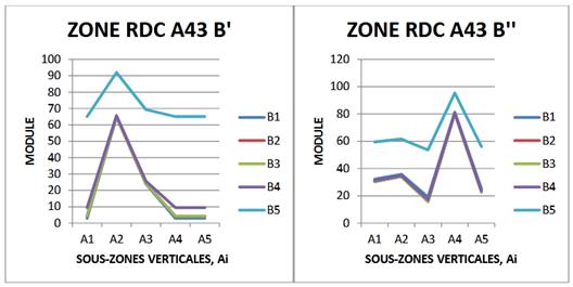
-The two
structures below have the same shape or mode with concavity facing upwards, but
symmetrical: the final part of the curves of one is worth the initial part for
the other and vice versa; simply turn one over and superimpose it on the other
to have identical structures.
Figure 8a: comparison of the structural curves of zones A43B' and A43B''
What has just been observed above is also valid for
the two structures below.
NB: A42 (Virunga-Kivu) and
A43 (Tanganyika).
Figure 8b: comparison of the structure curves of zones A42T and A43T
We observe that the structure of zone A44 (Upemba rift zone, Haut-Katanga region) straddles A42T and
A43T. These nuances are also observed in relation to the orientations of the
main faults (Figure 9).
Figure 8c: comparison of the structural curves of zones A44T and A51T
Overall its two structures below are the opposite of
one (concavity upwards) of the other (concavity downwards);
Figure 8d: comparison of the structure curves of zones A52T and A53T
The following two structures are so similar that we
can affirm that the entire structure of the DRC (10-35°E, 6°N-14°S) is dictated
by that of the A42B'' zone (Virunga zone at depth
exceeding 30km);
Figure 8e: comparison of the structure curves of the A4B'' zones and the
DRC (all)
These two structures below are similar, yet we
observed that their total structures (A42T and A43T, figure 8b) are opposite or
symmetrical; this shows that the orientations of the main faults of these two
zones are sometimes parallel, sometimes crossed at certain depths (Figure 9).
Figure 8f: comparison of the structural curves of zones A43G and A42B
Indeed, the geological overview of the DRC shows that
this territory has the following characteristics (Figure 1 and 9):
-In the eastern
part of the western branch of the East African Rift system, a network of main
faults winds from north to south, from Lake Albert in the north to Lake
Tanganyika in the south. From the southern end of Lake Tanganyika, the fault
system extends in a southwest direction towards Lake Moero
and Lake Upemba, then, in a southeast direction
towards Lake Rukwa and Malawi (Figure 2.3),
-Other faults
have been highlighted in the north-western part of the DRC, in the territory of
Ubangi, in the province of Equateur, and extends into the Central African
Republic, towards Bangui its capital,
-In the Kongo central province(Bas Congo),
in the west of the DRC, the structural map of the DRC highlights the presence
of faults; it is the same in the North-East of the DRC, in Orientale Province.
-However, Lake
Kivu is at the crossroads of two directions (South-West and South-East).
Figure 9: Structural map of the DRC (CRGM): the yellow lines represent the
main faults
3.2.4.6. Comparison of zones based on horizontal and vertical subzones
The comparison uses the following histograms
Figure 10a: Distribution of seismic levels of horizontal zones (Bj) by seismic zone A43
Figure 10b: Distribution of seismic levels of vertical zones (Ai) by
seismic zone A43
Figure 11a: Distribution of seismic levels of vertical zones (Ai) by
seismic zone A42
Figure 11b: Distribution of seismic levels of horizontal zones (Bj) by seismic zone A42
From these figures, we draw the following conclusions:
-A43T is similar
to A43C based on vertical subzones (Ai),
-A43T is similar
to A43C' based on the horizontal sub-zones (Bi),
-A42T is similar
to A42B based on vertical subzones (Ai),
-A42T is similar
to A42C based on horizontal subzones (Bi),
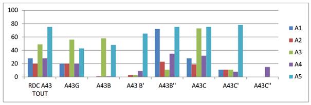
3.2.4.7. Final structures
The data in Table (12) and others in the appendix can
be grouped into classes; These include statistics on
the weight of each color (module) in the zoning maps (Figures 4). Table (21)
therefore groups the zones according to classes (in steps of fifteen); we
obtain six classes, one of which is empty
Indeed, we call
the modulus gap the difference between the maximum and minimum modulus of the
zone.
Table 21: classification of zones according to the gap relative to the
weight of the colors
-An exceptional
group including the zones of classes 1 and 2 with 14% of the zones: this group
only includes the derivatives of the zones of the Tanganyika region (A43 C''), Virunga-Lake Kivu (A42B') and the rift of Upemba-Haut Katanga (A44T),
-An intermediate group, 43%, made up of
classes 4 and 5: there we find the zones derived from A42 and A43, as well as
A42T and A43T,
-A final group
made up of class 6 which weighs 43%: this group includes all four zones between
30 and 35°E (A51T, A52T, A53T and A54T) and some derivatives of A42 and
A43
Overall, these criteria highlight a clear distinction
between the zones of the Congolese rift (A42, A43 and A44: 25-30°E) and that of
the Malawi-Zambezi rift (A51, A52, A53 A54: 30-35°E ).
The combination of the similarity rate, heterogeneity
and color gap parameters for each zone gives them the final structures
presented below
Figure 12a: Distribution of parameters in legend by
seismic zone
Observation of these structures (figure 10) groups
them into three classes;
Table 22: classification
of zones according to figure (10)
The analysis also integrating the heterogeneity rate
parameter based on the geo-seismic signature (figure 10b) highlights two
groups:
-One, composed
of areas located between 30 and 35°E (A51T, A52T, A53T and A54T),
-The other
consists of zones between 25 and 30°E (A42, A43 and A44T), in the Congolese
rift.
However,
depending on one or another parameter, these zones have some nuances:
vThe A44T zone (in the Upemba
rift) tends to separate from A42T (Virunga zone) to
get closer to A43T (Tanganyika zone),
vThe A42T zone, if not alone, is sometimes
close to the A5j zones. The A44T area seems to act as a hinge or suture zone
between the two groups ( ). The structural map (Figure 9) is in agreement with
the aforementioned observations, particularly with regard to the orientations
of the main faults (Figure 9).
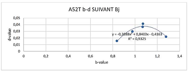
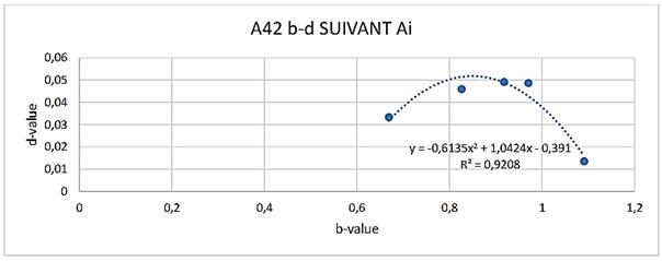
3.2.4.8. Comparison of zones based on b-value and d-value parameters
These parameters will allow us to model the structures
in order to follow the geodynamic evolution.
Remember that the b-value parameter measures the
seismic activity of an area, while the d-value measures the internal structure
(of the soil).
The search for the establishment of a correlation
between these two parameters provided the following curves.
Figure 13 a: Correlation between the b-value and the d-value for zone A51T
according to horizontal subdivisions
Figure 13 b: Correlation between the b-value and the d-value for zone A52T
according to horizontal subdivisions
Figure 13c: Correlation between the b-value and the
d-value for the A43T zone according to vertical subdivisions
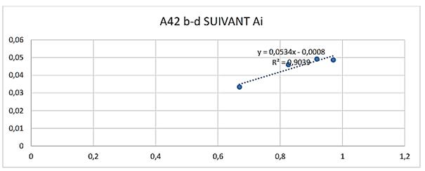
Figure 13 d: Linear correlation between the b-value and the d-value for the
A43T zone according to vertical subdivisions
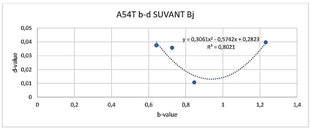
Figure 13e: Correlation between b-value and d-value for zone A54T based on
horizontal subdivisions
Figure 13f: Linear correlation between the b-value and the d-value for the
A42T zone according to the horizontal subdivisions
Figure 13g: Correlation between the b-value and the d-value for the A42T
zone according to vertical subdivisions
Figure 13h: Linear correlation between the b-value and the d-value for zone
42T according to horizontal subdivisions
Figure 13i: Correlation between the b-value and the d-value for the A53T
zone according to vertical subdivisions
Observation of the shapes of these curves reveals two
large families, one consisting of linear curves, the other of parabolic curves
(Table 23)
Table 23: classification of zones according to the shape of the correlation
curves
Shape of curves
curve
RIGHT
Positive concavity
Negativeconcavity
Positive slope
Negativeslope
Affected areas
A54T following
Ai
A51T next Bj
A52T next Bj
A53T next Bj
A42T following Ai
A42 following Ai
A42T next Bj
A43T following Ai
A42T following Ai
Analysis of the results in this table highlights the
following facts:
·The zones
located between 25 and 30°E, in the Congolese rift (A42, A43 and A44) have a
linear shape
·Those located
between 30 and 35°E, in the Malawi-Zambezi rift (A51, A52, A53 and A54) have a
parabolic shape,
·However, zones
A42T (Kivu zone) and A54T (Malawi zone) have nuanced trends (exceptions),
therefore straddling the two previous groups.
3.3. Location of main faults
The location of underground faults is often done by
exploiting the gravity and geomagnetic data of the region (Mbata,
2023; Ngindu, 2021; Mulopo,
2023; Tondozi, 2018). As far as we are concerned, the
interest is focused on the location of said faults by exploiting the
fundamental data of seismic activity.
To do this, this
location will be based on the hypothesis that: “the main underground faults are
located in places where the seismic activity module is at its peak”. This
paroxysm corresponds in figure (7) to the zone where the modulus is the
highest; which gives rise to the results contained in Figures (14-15) for zones
A42 and A43.
Figure 14: Location of main and minor faults in the Aij
zone
Reading Figure (14) responds to the legend above:
·Red color: the
main fault is located in layer G (0-10 km)
·Yellow color:
the main fault is located in layer C (10-20 km),
·Green color:
the main fault is located in layer C' (20-40 km),
·Blue color: the
main fault is located in layer C'' (>40 km),
·Purple color:
the main fault is located in the C' and C'' layer, therefore (>20 km),
·White color: no
main fault, but minor faults can be found.
The comparative analysis of these results reveals the
following:
·For both zone
A42 and zone A43, no main fault was observed in zone A4; this zone is therefore
the most stable.
·While the
position of the main faults at layer G (0-10 km) is located at A5 for seismic
zone A42, these faults are located at zone A3 for A43 for the same layer (G)
and the opposite at the layer C (10-20 km); this observation could be explained
by:
vThe heterogeneity of the soil above 20 km,
vThe position of two zones: zone A42,
including Lake Kivu, is located at a height of 1462 km and a depth of 485 km. The
A43 zone, including Lake Tanganyika, is located at a height of 780 km and a
depth of 1433 km,
vThe orientation of the faults in these two
zones are opposite (Figure 1,2 and 9): NW-SE
orientation for Lake Tanganyika (Bopili, 2009) and
NE-SW for Lake Kivu .
We note a sort of alternation or compensation in the
geodynamics between the two zones
towards regions close to
the rift at a depth not exceeding 20 km,
Beyond twenty kilometers in depth, the main faults are
almost, for both A42 and A43, located on A1; which means that
:
vFrom the surface to a depth of 20 km, the
faults are close to the rift, moving away from it beyond the depth of 20 km
(position of the Conrad discontinuity),
vThe soil structure is more homogeneous and
denser beyond 20 km than above, in accordance with the literature ( ),
In short, we conclude by saying that the
characterization scale designed is reasonable and that the hypothesis put
forward is also valid.
4. GENERAL CONCLUSION AND OUTLOOK
This research aims to highlight the fine structure of
the seismic zones of the western branch of the East African rift system using
the unified scale of characterization and the location of the main faults,
leading to the following conclusions:
Regarding the fine
structure, we note:
·Statistics on
seismic species discovered in the region show:
vIn total, we identified 89 seismic
species,
vThere are 28 (42%) seismic species common
to all areas,
vThere are 17% of species exclusive to
zones A51, A52, A52 and A54, zones between 20 and 25°E,
vThere are 17% of seismic species exclusive
to zone A42 subdivided into depth zones (A42G, A42B, A42B', A42B'', A42C,
A42C', A42C'') in the table (),
vThere are 17% of species exclusive to zone
A42 subdivided into depth zones (A42G, A42B, A42B', A42B'', A42C, A42C',
A42C'').
vThe average conservation rate of species
is 5%. We conclude that species are rarely preserved by going deep,
·Generally
speaking, all of these 21 zones align, depending on the color arrangements, on
one of two shapes:
vA symmetrical shape, these are A51T, A52T,
A52T and A54T, therefore the zones located between 20° and 25°E,
vA bipolar form (two groups of colors) for
all areas located between 25° and 20°E; these are the A42T, A42T, A44T and
their derivatives.
·From these
curves comparing the rate of resemblance to that of resemblance, the following
observations emerge:
vWith a few exceptions, there is a
correlation between the absolute resemblance rate and the relative resemblance
rate;
vWith a few exceptions, except at A42G and
A42B in the Virunga-Kivu region, there is a
correlation between the absolute or relative rate of resemblance and the rate
of heterogeneity,
vThere is a correlation between the number
of curves and the rate of heterogeneity; in fact, we see that the number of
curves decreases with the rate of heterogeneity: at less than 50% of this rate,
we have fewer than three structural curves.
vThe average rate of heterogeneity is 49%,
it is on average higher (55%) between 30 and 35°E and less between 25 and 30°E,
vthe combination of the three parameters
(rate of resemblance, heterogeneity and conservation of the species) brings
together 85% of the structures in the same class, the A42T zone (Virunga-Lake Kivu zone) being an exception and partially
the Tanganyika zone ( A43B'),
vWe observe that the structure of the A44
zone (Upemba rift zone, upper Katanga region)
straddles A42T (Virunga-Lake Kivu zone) and A43T
(Tanganyika zone), with implication on the orientation failures ,
vThere is reason to affirm that the
structure of the entire DRC is determined or predominated by that of the A42B''
zone (Virunga zone at a depth exceeding 30km).
·The analysis of the results based on the
b-alue and the d-value, one measuring seismic
activity, the other the soil structure, indicates that:
vThe zones located between 25 and 30°E, in
the Congolese rift (A42, A43 and A44) have a linear shape with some
particularities each,
vThose located between 30 and 35°E, in the
Malawi-Zambezi rift (A51, A52, A53 and A54) have a parabolic shape,
vHowever, zones A42T (Kivu zone) and A54T
(Malawi zone) have trends
vThe resemblance rate, based on structural
factors, between these two zones is 25%
vThe first zone is less seismic than the
second, one having a form factor (III), the other (IV)
vEach of these seven zones, whose
heterogeneity rate was 38% (Figure 2), no longer resembles itself alone;
therefore the heterogeneity rate increases to 100%
The location of the main faults is based on the
hypothesis that: “the main faults are located in places where the module of
seismic activity is at its peak”. The exploitation of this hypothesis and the
structure curves have:
·Made it
possible to locate the main and secondary faults,
·Shown that
going deeper, these faults change position; the shape is no longer vertical nor
rectilinear, but wavy and serpentine,
·Showed that
these results are in accordance with field observations and literature
·allowed us to
note that from the surface to a depth of 20 km, the faults of the Kivu (A42)
and Tanganyika (A43) zones are located near the rift, to move away from it
beyond the depth of 20 km ( corresponding to the average position of the Conrad
discontinuity),
·While the
position of the main faults at layer G (0-10 km) is located at A5 for seismic
zone A42, these faults are located at zone A3 for A43 for the same layer (G)
and the opposite at the layer C (10-20 km) and are all located at A1 beyond 20
km,
In short, we say that our model based on the discovery
of seismic species and the generation of the characterization scale is
reasonable and that the hypothesis put forward is valid. Indeed, their
exploitation has allowed a better characterization, both quantitative and
qualitative, of the soil structure and its geodynamics using fundamental
seismic parameters. Theseresults go beyondwhatisknown.
REFERENCES
1.Bantidi M., Wafula
M., Mavambou, Mukange B., ZanaNd., (2014a). Probabilistic assessment of seismic hazard in
Lake Tanganyika Rift accounting for local geologies conditions. 2015. International Journal of Geology,
Agriculture and Environmental Sciences. Vol.03 Issue 02 (April 2015),
pp24-29.
2.Bantidi
M., Mukange B., et Zana N.,
(2014b). Structure de la sismicité de la Branche occidentale des Rifts Valleys du système des Rifts Est-africains ; de 1954 à
2010, International Journal of Innovation
and AppliedStudies,
ISSN 2028-9324 Vol. 9 No. 4 Dec. 2014, pp.1562-1581.
3.Biliki
K;.and al.,(2021). Interpretation of Gravity Data and Contribution to the
Study of the Geological Structure of the Province of Mai-Ndombe
in DR. Congo: Implications in the Exploration of Hydrocarbons.
International Journal of Innovative Science and Research Technology, Volume 6, Issue 4, April – 2021, pp213-921.
4.Borden J-P., (1988). Biologie-Géologie. Première S. Paris: Bordas
5.Bopili M.L., (2009). Etudes des fluctuations de la température et
de la vitesse des vents au lac Tanganyika (une analysepar ondelettes). Thèse de doctorat :
Université de Kinshasa, Faculté des Sciences, Département de Physique. pp. 9-28
6.Lay T., and Wallace T., (1995). Modern Global seismology. New-York : Academic Press
7.MavongaTuluka
G., (2009).Seismic hazard assessment and
volcanogenic seismicity for the Democratic Republic of Congo and surrounding
areas, western Rift valley of Africa. Thèse de Doctorat: University of the Witwatersrand (Johannesburg),
Faculty of Sciences.
8.Mbata A. and al., (2023). A
comparative structural study of Southern region shallow basement of the
North-Kivu Province (DR. Congo) by gravity and magnetic data analysis. Journal
of Geoscience and environnement protection, Vol 11, pp 90-117.https://
doi.org/10.4236/gep.2023.119007.
9.Mukange B., Bantidi
M., ZanaNd., (2013). Structure de
la sismicité de la Branche orientale des Rifts Valleys
du système des Rifts Est-africains ; de 1954 à 2010. Revue Congolaise des Sciences Nucléaires. vol.27, pp151-169.
10.Mukange B., Bantidi
M., Zana L., Wafula M., ZanaNd., (2015). The isoseismal map and
their implication to underlining ground degree of heterogeneity (Kabalo quake’s case, September 11, 1992, magnitude 6.7, Upemba Rift). Greener
Journal of Geology and Earth Sciences, vol. 3 (2), pp
030-042.
11.Mukange B., (2016). Conception d’un modèle physique pour la caractérisationet la surveillance de l’activité sismique et
son implication géologique(Cas de la République Démocratique du Congo).
Thèse de Doctorat : Université de Kinshasa,Faculté des Sciences. Département de Physique.
12.MukangeBesa, (2021). Cours de Géophysique générale.
Université de Kinshasa, Faculté des Sciences.
13.Mukange B., (2021a).Design of a unified scale for the
characterization of seismic activity. International Journal of Innovative
Science and Research Technology, Volume 6, Issue 7 ,
July– 2021, pp.1407-1422. www.ijisrt.com
14.Mukange B., (2021b).Application of the unified scale to
the characterization of seismic activity of the Democratic Republic of Congo
and its surroundings (comparative study for Africa, Indonesia and the Pacific
coast of Central America). International Journal of Innovative Science and
Research Technology, Volume 6, Issue 7, July– 2021, pp.1516-1555.
www.ijisrt.com
15.Mukange B.,
(2023a). Characterization of the volcano-seismic activity around Nyiragongo volcano and location of its crater by means of
unified scale. Greener Journal of Geology
and Earth Sciences, 5(1) December 2023: 28-51.
http//gjournals.org/GJGES.
16.Mukange B., (2023b). Characterization of the volcano-seismic
activity around Nyamulagira volcano and
location of its crater by means of unified scale. Greener Journal of Geology and Earth Sciences, 5(1) December 2023: 52-75. http//gjournals.org/GJGES.
17.Mulopo, (2023). Analyse
des corrélations entre les linéaments et les accidents tectoniques de la région
de Lubumbashi-Kipushi : contribution à l’étude
classique de la tectonique régionale en République Démocratique du Congo.
Thèse de Doctorat : Université Pédagogique Nationale, Faculté des Sciences.
Département de Physique
18.Musitu
M. and al., (2023). Structural mapping of Kakobola
and its surroundings by analyzing geomagnetic data. Journal
of Geoscience and environnement protection, Vol 11,
pp 64-89.https:// doi.org/10.4236/gep.2023.119006.
19.Ngindu
D. and al., (2021). New Faults from the Geodynamics of South Katanga in D.R.Congo.International Journal of Innovative Science and Research Technology, Vol(6)
Issue 1(January 2021),pp1596-1689.
20.Tondozi K. and al, (2018). Interpretation of
gravity anomalies maps and contribution to the structural study of a
sedimentary basin of major petroleum interest: Case of the Busira
sub-basin in the Central basin of the DR Congo, IJIAS Vol. 24 N°1, p. 68-88.
Cite this Article: Mukange, BA; Katwika,
C; Jalum, B; Zana, NA; Tondozi, KF (2023). Highlighting
the Fine Structure of the Seismic Zones of the
Western Branch of the East African
Rift System Using the UnifiedCharacterizationScale
and ItsGeological
Implication.Greener Journal of Geology
and Earth Sciences, 5(1): 76-108.